
'How do neural nets learn?' A step by step explanation using the H2O Deep Learning algorithm.
In my last blogpost about Random Forests I introduced the codecentric.ai Bootcamp. The next part I published was about Neural Networks and Deep Learning. Every video of our bootcamp will have example code and tasks to promote hands-on learning. While the practical parts of the bootcamp will be using Python, below you will find the English R version of this Neural Nets Practical Example, where I explain how neural nets learn and how the concepts and techniques translate to training neural nets in R with the H2O Deep Learning function.
You can find the video on YouTube but as, as before, it is only available in German. Same goes for the slides, which are also currently German only. See the end of this article for the embedded video and slides.
Neural Nets and Deep Learning
Just like Random Forests, neural nets are a method for machine learning and can be used for supervised, unsupervised and reinforcement learning. The idea behind neural nets has already been developed back in the 1940s as a way to mimic how our human brain learns. That’s way neural nets in machine learning are also called ANNs (Artificial Neural Networks).
When we say Deep Learning, we talk about big and complex neural nets, which are able to solve complex tasks, like image or language understanding. Deep Learning has gained traction and success particularly with the recent developments in GPUs and TPUs (Tensor Processing Units), the increase in computing power and data in general, as well as the development of easy-to-use frameworks, like Keras and TensorFlow. We find Deep Learning in our everyday lives, e.g. in voice recognition, computer vision, recommender systems, reinforcement learning and many more.
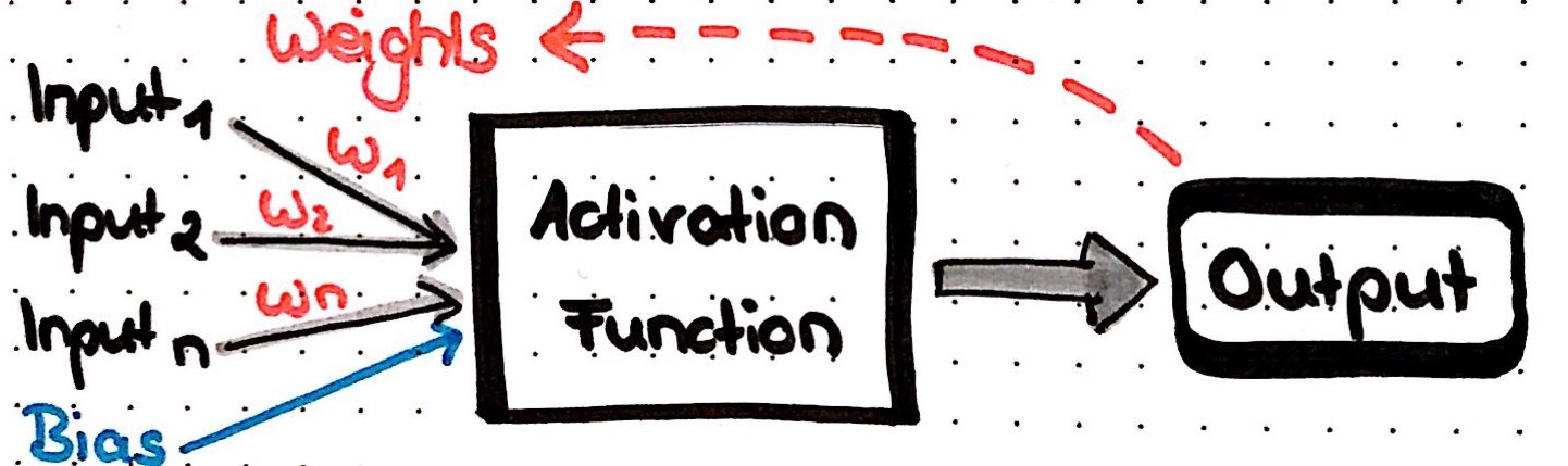
The easiest type of ANN has only node (also called neuron) and is called perceptron. Incoming data flows into this neuron, where a result is calculated, e.g. by summing up all incoming data. Each of the incoming data points is multiplied with a weight; weights can basically be any number and are used to modify the results that are calculated by a neuron: if we change the weight, the result will change also. Optionally, we can add a so called bias to the data points to modify the results even further.
But how do neural nets learn? Below, I will show with an example that uses common techniques and principles.
Libraries
First, we will load all the packages we need:
- tidyverse for data wrangling and plotting
- readr for reading in a csv
- h2o for Deep Learning (
h2o.initinitializes the cluster)
library(tidyverse)
library(readr)
library(h2o)
h2o.init(nthreads = -1)
##
## H2O is not running yet, starting it now...
##
## Note: In case of errors look at the following log files:
## /var/folders/5j/v30zfr7s14qfhqwqdmqmpxw80000gn/T//Rtmp6br9Lr/h2o_shiringlander_started_from_r.out
## /var/folders/5j/v30zfr7s14qfhqwqdmqmpxw80000gn/T//Rtmp6br9Lr/h2o_shiringlander_started_from_r.err
##
##
## Starting H2O JVM and connecting: ... Connection successful!
##
## R is connected to the H2O cluster:
## H2O cluster uptime: 2 seconds 427 milliseconds
## H2O cluster timezone: Europe/Berlin
## H2O data parsing timezone: UTC
## H2O cluster version: 3.22.1.1
## H2O cluster version age: 28 days and 42 minutes
## H2O cluster name: H2O_started_from_R_shiringlander_xnf724
## H2O cluster total nodes: 1
## H2O cluster total memory: 3.56 GB
## H2O cluster total cores: 8
## H2O cluster allowed cores: 8
## H2O cluster healthy: TRUE
## H2O Connection ip: localhost
## H2O Connection port: 54321
## H2O Connection proxy: NA
## H2O Internal Security: FALSE
## H2O API Extensions: XGBoost, Algos, AutoML, Core V3, Core V4
## R Version: R version 3.5.2 (2018-12-20)Data
The dataset used in this example is a customer churn dataset from Kaggle.
Each row represents a customer, each column contains customer’s attributes
We will load the data from a csv file:
telco_data <- read_csv("../../../Data/Churn/WA_Fn-UseC_-Telco-Customer-Churn.csv")## Parsed with column specification:
## cols(
## .default = col_character(),
## SeniorCitizen = col_double(),
## tenure = col_double(),
## MonthlyCharges = col_double(),
## TotalCharges = col_double()
## )## See spec(...) for full column specifications.head(telco_data)## # A tibble: 6 x 21
## customerID gender SeniorCitizen Partner Dependents tenure PhoneService
## <chr> <chr> <dbl> <chr> <chr> <dbl> <chr>
## 1 7590-VHVEG Female 0 Yes No 1 No
## 2 5575-GNVDE Male 0 No No 34 Yes
## 3 3668-QPYBK Male 0 No No 2 Yes
## 4 7795-CFOCW Male 0 No No 45 No
## 5 9237-HQITU Female 0 No No 2 Yes
## 6 9305-CDSKC Female 0 No No 8 Yes
## # … with 14 more variables: MultipleLines <chr>, InternetService <chr>,
## # OnlineSecurity <chr>, OnlineBackup <chr>, DeviceProtection <chr>,
## # TechSupport <chr>, StreamingTV <chr>, StreamingMovies <chr>,
## # Contract <chr>, PaperlessBilling <chr>, PaymentMethod <chr>,
## # MonthlyCharges <dbl>, TotalCharges <dbl>, Churn <chr>Let’s quickly examine the data by plotting density distributions of numeric variables…
telco_data %>%
  select_if(is.numeric) %>%
  gather() %>%
  ggplot(aes(x = value)) +
    facet_wrap(~ key, scales = "free", ncol = 4) +
    geom_density()
## Warning: Removed 11 rows containing non-finite values (stat_density).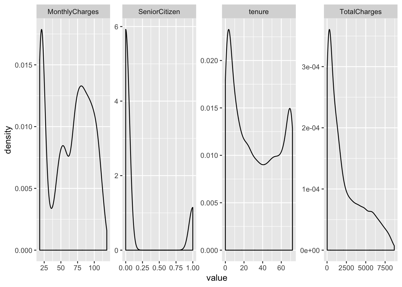
… and barcharts for categorical variables.
telco_data %>%
  select_if(is.character) %>%
  select(-customerID) %>%
  gather() %>%
  ggplot(aes(x = value)) +
    facet_wrap(~ key, scales = "free", ncol = 3) +
    geom_bar()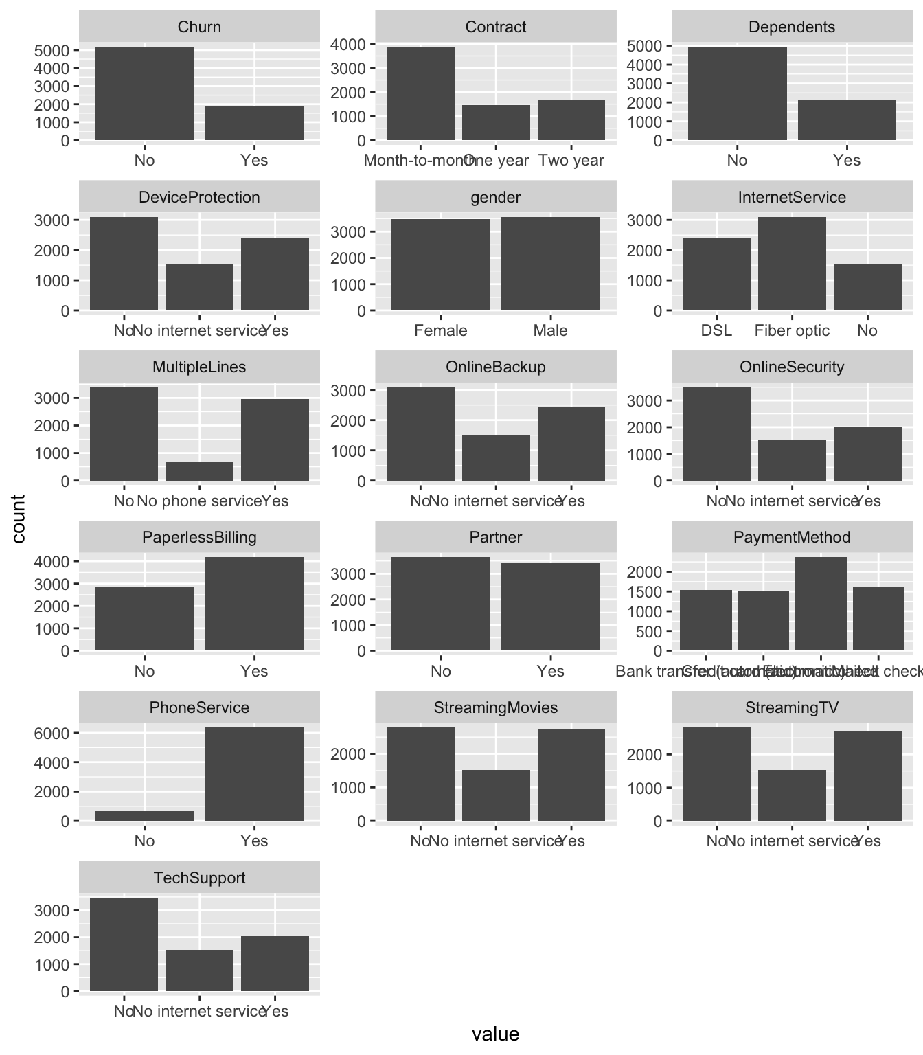
Before we can work with h2o, we need to convert our data into an h2o frame object. Note, that I am also converting character columns to categorical columns, otherwise h2o will ignore them. Moreover, we will need our response variable to be in categorical format in order to perform classification on this data.
hf <- telco_data %>%
  mutate_if(is.character, as.factor) %>%
  as.h2o
Next, I’ll create a vector of the feature names I want to use for modeling (I am leaving out the customer ID because it doesn’t add useful information about customer churn).
hf_X <- colnames(telco_data)[2:20]
hf_X
## [1] "gender" "SeniorCitizen" "Partner"
## [4] "Dependents" "tenure" "PhoneService"
## [7] "MultipleLines" "InternetService" "OnlineSecurity"
## [10] "OnlineBackup" "DeviceProtection" "TechSupport"
## [13] "StreamingTV" "StreamingMovies" "Contract"
## [16] "PaperlessBilling" "PaymentMethod" "MonthlyCharges"
## [19] "TotalCharges"I am doing the same for the response variable:
hf_y <- colnames(telco_data)[21]
hf_y
## [1] "Churn"Now, we are ready to use the h2o.deeplearning function, which has a number of arguments and hyperparameters, which we can set to define our neural net and the learning process. The most essential arguments are
y: the name of the response variabletraining_frame: the training datax: the vector of features to use is optional and all remaining columns would be used if we don’t specify it, but since we don’t want to include customer id in our model, we need to give this vector here.
The H2O documentation for the Deep Learning function gives an overview over all arguments and hyperparameters you can use. I will explain a few of the most important ones.
dl_model <- h2o.deeplearning(x = hf_X,
                             y = hf_y,
                             training_frame = hf)
Activation functions
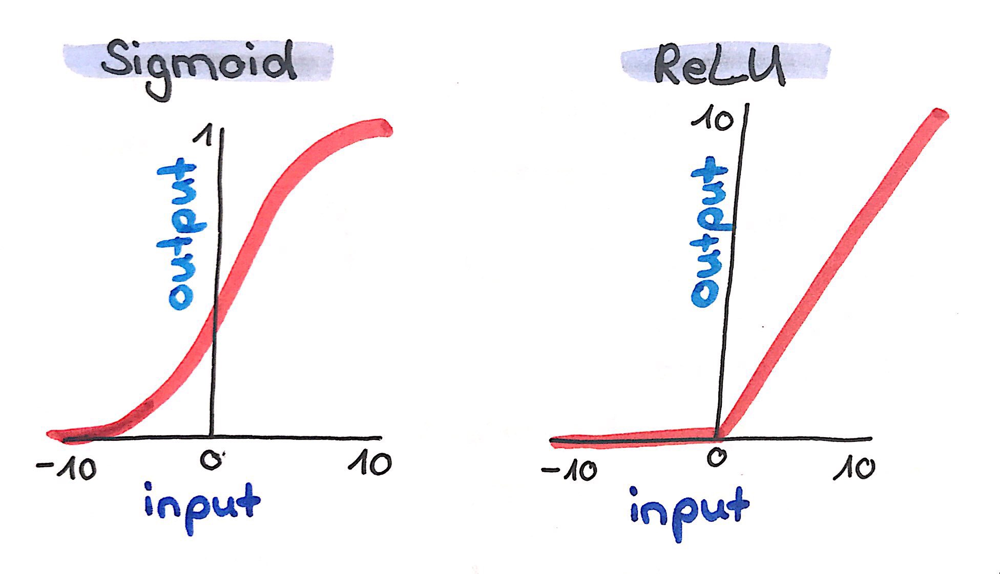
Before, when describing the simple perceptron, I said that a result is calculated in a neuron, e.g. by summing up all the incoming data multiplied by weights. However, this has one big disadvantage: such an approach would only enable our neural net to learn linear relationships between data. In order to be able to learn (you can also say approximate) any mathematical problem - no matter how complex - we use activation functions. Activation functions normalize the output of a neuron, e.g. to values between -1 and 1, (Tanh), 0 and 1 (Sigmoid) or by setting negative values to 0 (Rectified Linear Units, ReLU). In H2O we can choose between Tanh, Tanh with Dropout, Rectifier (default), Rectifier with Dropout, Maxout and Maxout with Dropout. Let’s choose Rectifier with Dropout. Dropout is used to improve the generalizability of neural nets by randomly setting a given proportion of nodes to 0. The dropout rate in H2O is specified with two arguments: hidden_dropout_ratios, which per default sets 50% of hidden (more on that in a minute) nodes to 0. Here, I want to reduce that proportion to 20% but let’s talk about hidden layers and hidden nodes first. In addition to hidden dropout, H2O let’s us specify a dropout for the input layer with input_dropout_ratio. This argument is deactivated by default and this is how we will leave it.
dl_model <- h2o.deeplearning(x = hf_X,
                             y = hf_y,
                             training_frame = hf,
                             activation = "RectifierWithDropout")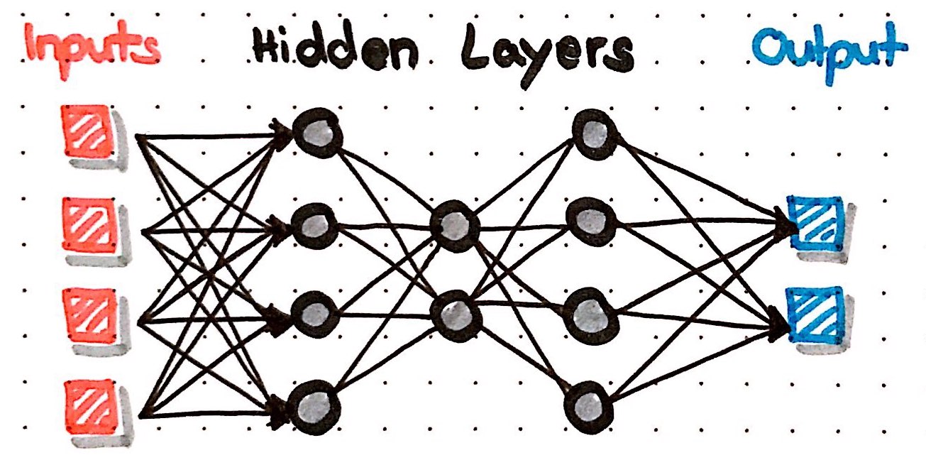
Learning through optimisation
Just as in the simple perceptron from the beginning, our MLP has weights associated with every node. And just as in the simple perceptron, we want to find the most optimal combination of weights in order to get a desired result from the output layer. The desired result in a supervised learning task is for the neural net to calculate predictions that are as close to reality as possible.
How that works has a lot to do with mathematical optimization and the following concepts:
- difference between prediction and reality
- loss functions
- backpropagation
- optimization methods, like gradient descent
Difference between prediction and reality
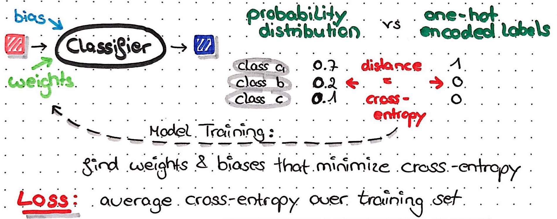
When our network calculates a predictions, what the output nodes will return before applying an activation function is a numeric value of any size - this is called the score. Just as before, we will now apply an activation function to this score in order to normalize it. In the output of a classification task, we would like to get values between 0 and 1, that’s why we most commonly use the softmax function; this function converts the scores for every possible outcome/class into a probability distribution with values between 0 and 1 and a sum of 1.
One-Hot-Encoding
In order to compare this probability distribution of predictions with the true outcome/class, we use a special format to encode our outcome: One-Hot-Encoding. For every instance, we will generate a vector with either 0 or 1 for every possible class: the true class of the instance will get a 1, all other classes will get 0s. This one-hot-encoded vector now looks very similar to a probability distribution: it contains values between 0 and 1 and sums up to 1. In fact, our one-hot-encoded vector looks like the probability distribution if our network had predicted the correct class with 100% certainty!
We can now use this similarity between probability distribution and one-hot-encoded vector to calculate the difference between the two; this difference tells us how close to reality our network is: if the difference is small, it is close to reality, if the difference is big, it wasn’t very accurate in predicting the outcome. The goal of the learning process is now to find the combination of weights that make the difference between probability distribution and one-hot-encoded vector as small as possible.
One-Hot-Encoding will also be applied to categorical feature variables, because our neural nets need numeric values to learn from - strings and categories in their raw format are not useful per se. Fortunately, many machine learning packages - H2O being one of them - perform this one-hot-encoding automatically in the background for you. We could still change the categorical_encoding argument to “Enum”, “OneHotInternal”, “OneHotExplicit”, “Binary”, “Eigen”, “LabelEncoder”, “SortByResponse” and “EnumLimited” but we will leave the default setting of “AUTO”.
Loss-Functions
This minimization of the difference between prediction and reality for the entire training set is also called minimising the loss function. There are many different loss functions (and in some cases, you will even write your own specific loss function), in H2O we have “CrossEntropy”, “Quadratic”, “Huber”, “Absolute” and “Quantile”. In classification tasks, the loss function we want to minimize is usually cross-entropy.
dl_model <- h2o.deeplearning(x = hf_X,
                             y = hf_y,
                             training_frame = hf,
                             activation = "RectifierWithDropout",
                             hidden = c(100, 80, 100),
                             hidden_dropout_ratios = c(0.2, 0.2, 0.2),
                             loss = "CrossEntropy")
Backpropagation
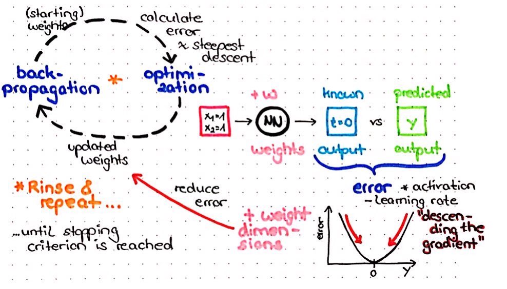
With backpropagation, the calculated error (from the cross entropy in our case) will be propagated back through the network to calculate the proportion of error for every neuron. Based on this proportion of error, we get an error landscape for every neuron. This error landscape can be thought of as a hilly landscape in the Alps, for example. The positions in this landscape are different weights, so that we get weights with high error at the peaks and weights with low error in valleys. In order to minimize the error, we want to find the position in this landscape (i.e. the weight) that is in the deepest valley.
Gradient descent
Let’s imagine we were a hiker, who is left at a random place in this landscape - while being blindfolded - and we are tasked with finding our way to this valley. We would start by feeling around and looking for the direction with the steepest downward slope. This is also what our neural net does, just that this “feeling around” is called “calculating the gradient”. And just as we would then make a step in that direction with the steepest downwards slope, our neural net makes a step in the direction with the steepest gradient. This is called gradient descent. This procedure will be repeated until we find a place, where we can’t go any further down. In our neural net, this number of repeated rounds is called the number of epochs and we define it in H2O with the epochs argument.
dl_model <- h2o.deeplearning(x = hf_X,
                             y = hf_y,
                             training_frame = hf,
                             activation = "RectifierWithDropout",
                             hidden = c(100, 80, 100),
                             hidden_dropout_ratios = c(0.2, 0.2, 0.2),
                             loss = "CrossEntropy",
                             epochs = 200)
Adaptive learning rate and momentum
One common problem with this simple approach is, that we might end up in a place, where there is no direction to go down any more but the steepest valley in the entire landscape is somewhere else. In our neural net, this would be called getting stuck in local minima or on saddle points. In order to be able to overcome these points and find the global minimum, several advanced techniques have been developed in recent years.
One of them is the adaptive learning rate. Learning rate can be though of as the step size of our hiker. In H2O, this is defined with the rate argument. With an adaptive learning rate, we can e.g. start out with a big learning rate reduce it the closer we get to the end of our model training run. If you wanted to have an adaptive learning rate in your neural net, you would use the following functions in H2O: adaptive_rate = TRUE, rho (rate of learning rate decay) and epsilon (a smoothing factor).
In this example, I am not using adaptive learning rate, however, but something called momentum. If you imagine a ball being pushed from some point in the landscape, it will gain momentum that propels it into a general direction and won’t make big jumps into opposing directions. This principle is applied with momentum in neural nets. In our H2O function we define momentum_start (momentum at the beginning of training), momentum_ramp (number of instances for which momentum is supposed to increase) and momentum_stable (final momentum).
The Nesterov accelerated gradient is an addition to momentum in which the next step is guessed before taking it. In this way, the previous error will influence the direction of the next step.
dl_model <- h2o.deeplearning(x = hf_X,
                             y = hf_y,
                             training_frame = hf,
                             activation = "RectifierWithDropout",
                             hidden = c(100, 80, 100),
                             hidden_dropout_ratios = c(0.2, 0.2, 0.2),
                             loss = "CrossEntropy",
                             epochs = 200,
                             rate = 0.005,
                             adaptive_rate = FALSE,
                             momentum_start = 0.5,
                             momentum_ramp = 100,
                             momentum_stable = 0.99,
                             nesterov_accelerated_gradient = TRUE)
L1 and L2 Regularization
In addition to dropout, we can apply regularization to improve the generalizability of our neural network. In H2O, we can use L1 and L2 regularization. With L1, many nodes will be set to 0 and with L2 many nodes will get low weights.
dl_model <- h2o.deeplearning(x = hf_X,
                             y = hf_y,
                             training_frame = hf,
                             activation = "RectifierWithDropout",
                             hidden = c(100, 80, 100),
                             hidden_dropout_ratios = c(0.2, 0.2, 0.2),
                             loss = "CrossEntropy",
                             epochs = 200,
                             rate = 0.005,
                             adaptive_rate = TRUE,
                             momentum_start = 0.5,
                             momentum_ramp = 100,
                             momentum_stable = 0.99,
                             nesterov_accelerated_gradient = TRUE,
                             l1 = 0,
                             l2 = 0)
Crossvalidation
Now you know the main principles of how neural nets learn!
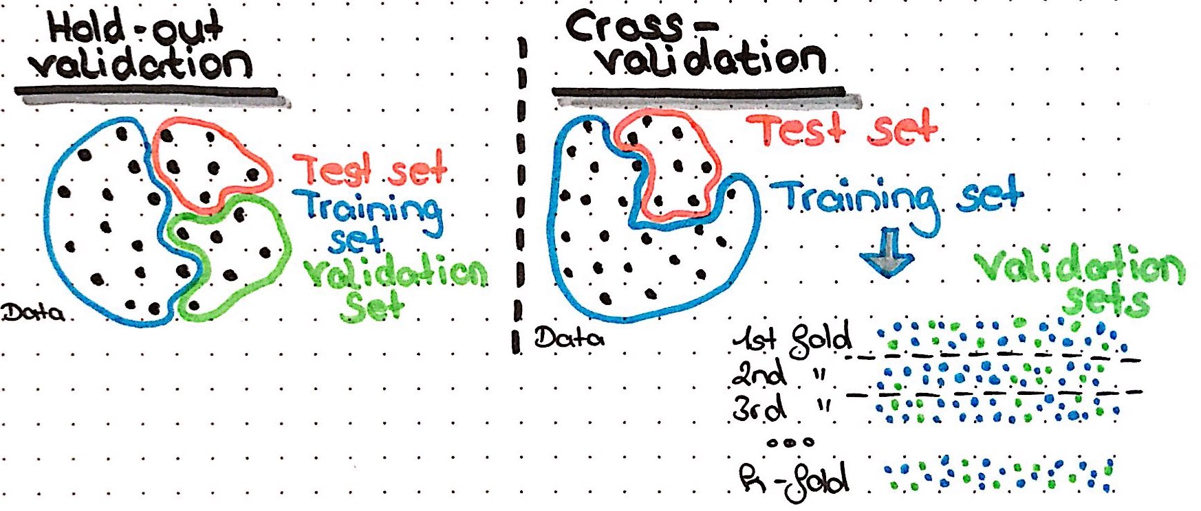
Before we finally train our model, we want to have a way to judge how well our model learned and if learning improves over the epochs. Here, we want to use validation data, to make these performance measures less biased compared to using the training data. In H2O, we could either give a specific validation set with validation_frame or we use crossvalidation. The argument nfolds specifies how many folds shall be generated and with fold_assignment = "Stratified" we tell H2O to make sure to keep the class ratios of our response variable the same in all folds. We also specify to save the cross validation predictions for examination.
dl_model <- h2o.deeplearning(x = hf_X,
                             y = hf_y,
                             training_frame = hf,
                             activation = "RectifierWithDropout",
                             hidden = c(100, 80, 100),
                             hidden_dropout_ratios = c(0.2, 0.2, 0.2),
                             loss = "CrossEntropy",
                             epochs = 200,
                             rate = 0.005,
                             adaptive_rate = FALSE,
                             momentum_start = 0.5,
                             momentum_ramp = 100,
                             momentum_stable = 0.99,
                             nesterov_accelerated_gradient = TRUE,
                             l1 = 0,
                             l2 = 0,
                             nfolds = 3,
                             fold_assignment = "Stratified",
                             keep_cross_validation_predictions = TRUE,
                             balance_classes = TRUE,
                             seed = 42)
Finally, we are balancing the class proportions and we set a seed for pseudo-number-generation - and we train our model!
The resulting model object can be used just like any other H2O model: for predicting new/test data, for calculating performance metrics, saving it, or plotting the training results:
plot(dl_model)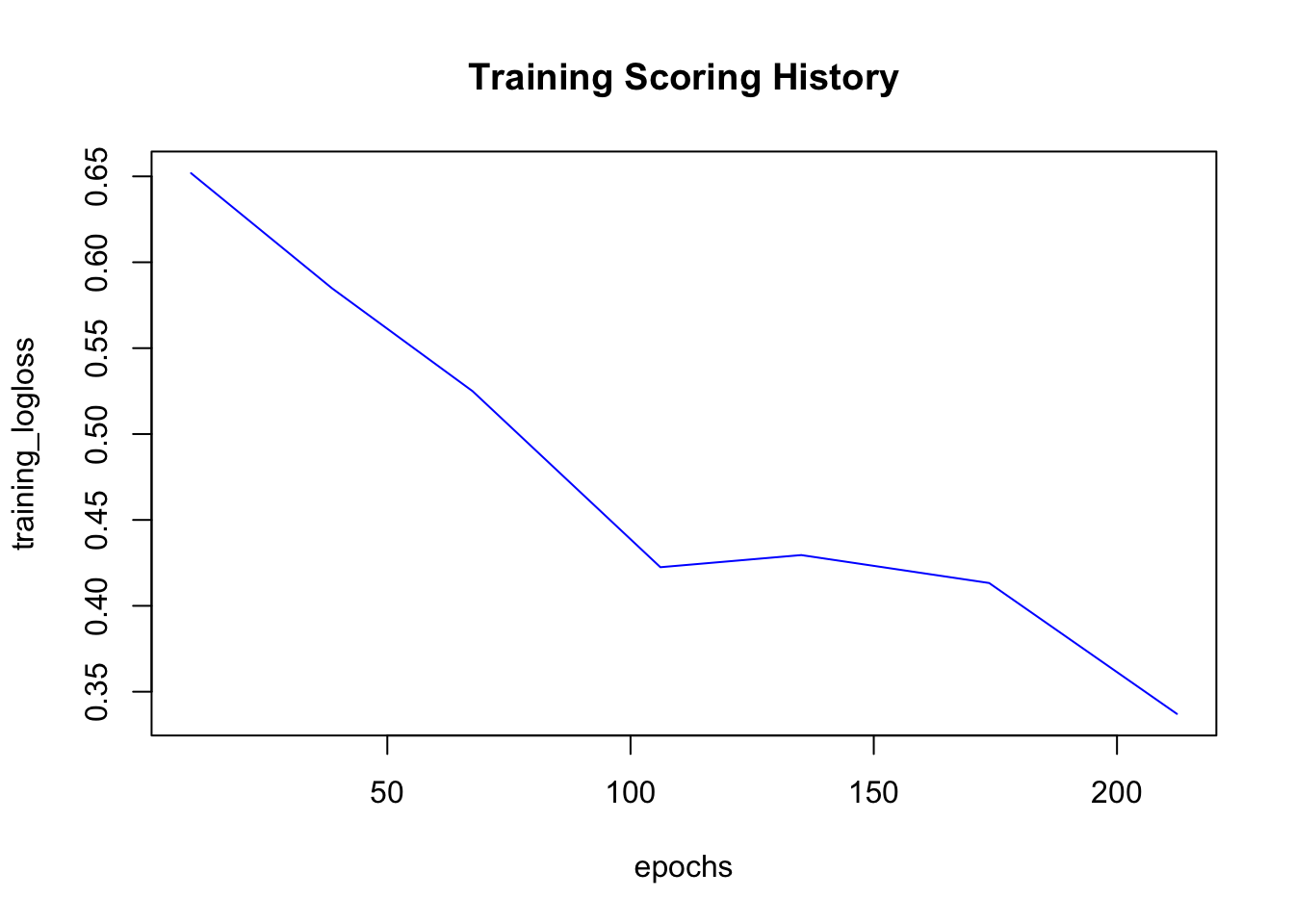
The crossvalidation predictions can be accessed with h2o.cross_validation_predictions() (returns one data frame for every fold) and h2o.cross_validation_holdout_predictions() (combined in one data frame).
h2o.cross_validation_predictions(dl_model)## [[1]]
## predict No Yes
## 1 No 0.0000000 0.00000000
## 2 No 0.9742401 0.02575991
## 3 No 0.0000000 0.00000000
## 4 No 0.9810427 0.01895733
## 5 Yes 0.1665065 0.83349348
## 6 Yes 0.1771927 0.82280726
##
## [7043 rows x 3 columns]
##
## [[2]]
## predict No Yes
## 1 Yes 0.4017627 0.5982373
## 2 No 0.0000000 0.0000000
## 3 No 0.8110977 0.1889023
## 4 No 0.0000000 0.0000000
## 5 No 0.0000000 0.0000000
## 6 No 0.0000000 0.0000000
##
## [7043 rows x 3 columns]
##
## [[3]]
## predict No Yes
## 1 No 0 0
## 2 No 0 0
## 3 No 0 0
## 4 No 0 0
## 5 No 0 0
## 6 No 0 0
##
## [7043 rows x 3 columns]h2o.cross_validation_holdout_predictions(dl_model)## predict No Yes
## 1 Yes 0.4017627 0.59823735
## 2 No 0.9742401 0.02575991
## 3 No 0.8110977 0.18890231
## 4 No 0.9810427 0.01895733
## 5 Yes 0.1665065 0.83349348
## 6 Yes 0.1771927 0.82280726
##
## [7043 rows x 3 columns]Video
Slides
sessionInfo()## R version 3.5.2 (2018-12-20)
## Platform: x86_64-apple-darwin15.6.0 (64-bit)
## Running under: macOS Mojave 10.14.2
##
## Matrix products: default
## BLAS: /Library/Frameworks/R.framework/Versions/3.5/Resources/lib/libRblas.0.dylib
## LAPACK: /Library/Frameworks/R.framework/Versions/3.5/Resources/lib/libRlapack.dylib
##
## locale:
## [1] en_US.UTF-8/en_US.UTF-8/en_US.UTF-8/C/en_US.UTF-8/en_US.UTF-8
##
## attached base packages:
## [1] stats graphics grDevices utils datasets methods base
##
## other attached packages:
## [1] bindrcpp_0.2.2 h2o_3.22.1.1 forcats_0.3.0 stringr_1.3.1
## [5] dplyr_0.7.8 purrr_0.2.5 readr_1.3.1 tidyr_0.8.2
## [9] tibble_2.0.1 ggplot2_3.1.0 tidyverse_1.2.1
##
## loaded via a namespace (and not attached):
## [1] tidyselect_0.2.5 xfun_0.4 haven_2.0.0 lattice_0.20-38
## [5] colorspace_1.4-0 generics_0.0.2 htmltools_0.3.6 yaml_2.2.0
## [9] utf8_1.1.4 rlang_0.3.1 pillar_1.3.1 glue_1.3.0
## [13] withr_2.1.2 modelr_0.1.2 readxl_1.2.0 bindr_0.1.1
## [17] plyr_1.8.4 munsell_0.5.0 blogdown_0.10 gtable_0.2.0
## [21] cellranger_1.1.0 rvest_0.3.2 evaluate_0.12 labeling_0.3
## [25] knitr_1.21 fansi_0.4.0 broom_0.5.1 Rcpp_1.0.0
## [29] scales_1.0.0 backports_1.1.3 jsonlite_1.6 hms_0.4.2
## [33] digest_0.6.18 stringi_1.2.4 bookdown_0.9 grid_3.5.2
## [37] bitops_1.0-6 cli_1.0.1 tools_3.5.2 magrittr_1.5
## [41] lazyeval_0.2.1 RCurl_1.95-4.11 crayon_1.3.4 pkgconfig_2.0.2
## [45] xml2_1.2.0 lubridate_1.7.4 assertthat_0.2.0 rmarkdown_1.11
## [49] httr_1.4.0 rstudioapi_0.9.0 R6_2.3.0 nlme_3.1-137
## [53] compiler_3.5.2