
Code for case study - Customer Churn with Keras/TensorFlow and H2O
This is code that accompanies a book chapter on customer churn that I have written for the German dpunkt Verlag. The book is in German and will probably appear in February: https://www.dpunkt.de/buecher/13208/9783864906107-data-science.html.
The code you find below can be used to recreate all figures and analyses from this book chapter. Because the content is exclusively for the book, my descriptions around the code had to be minimal. But I’m sure, you can get the gist, even without the book. ;-)
Inspiration & Sources
Thank you to the following people for providing excellent code examples about customer churn:
Setup
All analyses are done in R using RStudio. For detailed session information including R version, operating system and package versions, see the sessionInfo() output at the end of this document.
All figures are produced with ggplot2.
- Libraries
# Load libraries
library(tidyverse) # for tidy data analysis
library(readr)     # for fast reading of input files
library(caret)     # for convenient splitting
library(mice)      # mice package for Multivariate Imputation by Chained Equations (MICE)
library(keras)     # for neural nets
library(lime)      # for explaining neural nets
library(rsample)   # for splitting training and test data
library(recipes)   # for preprocessing
library(yardstick) # for evaluation
library(ggthemes)  # for additional plotting themes
library(corrplot)  # for correlation

theme_set(theme_minimal())
# Install Keras if you have not installed it before
# follow instructions if you haven't installed TensorFlow
install_keras()Data preparation
The dataset
The Telco Customer Churn data set is the same one that Matt Dancho used in his post (see above). It was downloaded from IBM Watson
churn_data_raw <- read_csv("WA_Fn-UseC_-Telco-Customer-Churn.csv")glimpse(churn_data_raw)## Observations: 7,043
## Variables: 21
## $ customerID <chr> "7590-VHVEG", "5575-GNVDE", "3668-QPYBK", "77...
## $ gender <chr> "Female", "Male", "Male", "Male", "Female", "...
## $ SeniorCitizen <dbl> 0, 0, 0, 0, 0, 0, 0, 0, 0, 0, 0, 0, 0, 0, 0, ...
## $ Partner <chr> "Yes", "No", "No", "No", "No", "No", "No", "N...
## $ Dependents <chr> "No", "No", "No", "No", "No", "No", "Yes", "N...
## $ tenure <dbl> 1, 34, 2, 45, 2, 8, 22, 10, 28, 62, 13, 16, 5...
## $ PhoneService <chr> "No", "Yes", "Yes", "No", "Yes", "Yes", "Yes"...
## $ MultipleLines <chr> "No phone service", "No", "No", "No phone ser...
## $ InternetService <chr> "DSL", "DSL", "DSL", "DSL", "Fiber optic", "F...
## $ OnlineSecurity <chr> "No", "Yes", "Yes", "Yes", "No", "No", "No", ...
## $ OnlineBackup <chr> "Yes", "No", "Yes", "No", "No", "No", "Yes", ...
## $ DeviceProtection <chr> "No", "Yes", "No", "Yes", "No", "Yes", "No", ...
## $ TechSupport <chr> "No", "No", "No", "Yes", "No", "No", "No", "N...
## $ StreamingTV <chr> "No", "No", "No", "No", "No", "Yes", "Yes", "...
## $ StreamingMovies <chr> "No", "No", "No", "No", "No", "Yes", "No", "N...
## $ Contract <chr> "Month-to-month", "One year", "Month-to-month...
## $ PaperlessBilling <chr> "Yes", "No", "Yes", "No", "Yes", "Yes", "Yes"...
## $ PaymentMethod <chr> "Electronic check", "Mailed check", "Mailed c...
## $ MonthlyCharges <dbl> 29.85, 56.95, 53.85, 42.30, 70.70, 99.65, 89....
## $ TotalCharges <dbl> 29.85, 1889.50, 108.15, 1840.75, 151.65, 820....
## $ Churn <chr> "No", "No", "Yes", "No", "Yes", "Yes", "No", ...EDA
- Proportion of churn
churn_data_raw %>%
  count(Churn)
## # A tibble: 2 x 2
## Churn n
## <chr> <int>
## 1 No 5174
## 2 Yes 1869- Plot categorical features
churn_data_raw %>%
  mutate(SeniorCitizen = as.character(SeniorCitizen)) %>%
  select(-customerID) %>%
  select_if(is.character) %>%
  select(Churn, everything()) %>%
  gather(x, y, gender:PaymentMethod) %>%
  count(Churn, x, y) %>%
  ggplot(aes(x = y, y = n, fill = Churn, color = Churn)) +
    facet_wrap(~ x, ncol = 4, scales = "free") +
    geom_bar(stat = "identity", alpha = 0.5) +
    theme(axis.text.x = element_text(angle = 90, hjust = 1),
          legend.position = "top") +
    scale_color_tableau() +
    scale_fill_tableau()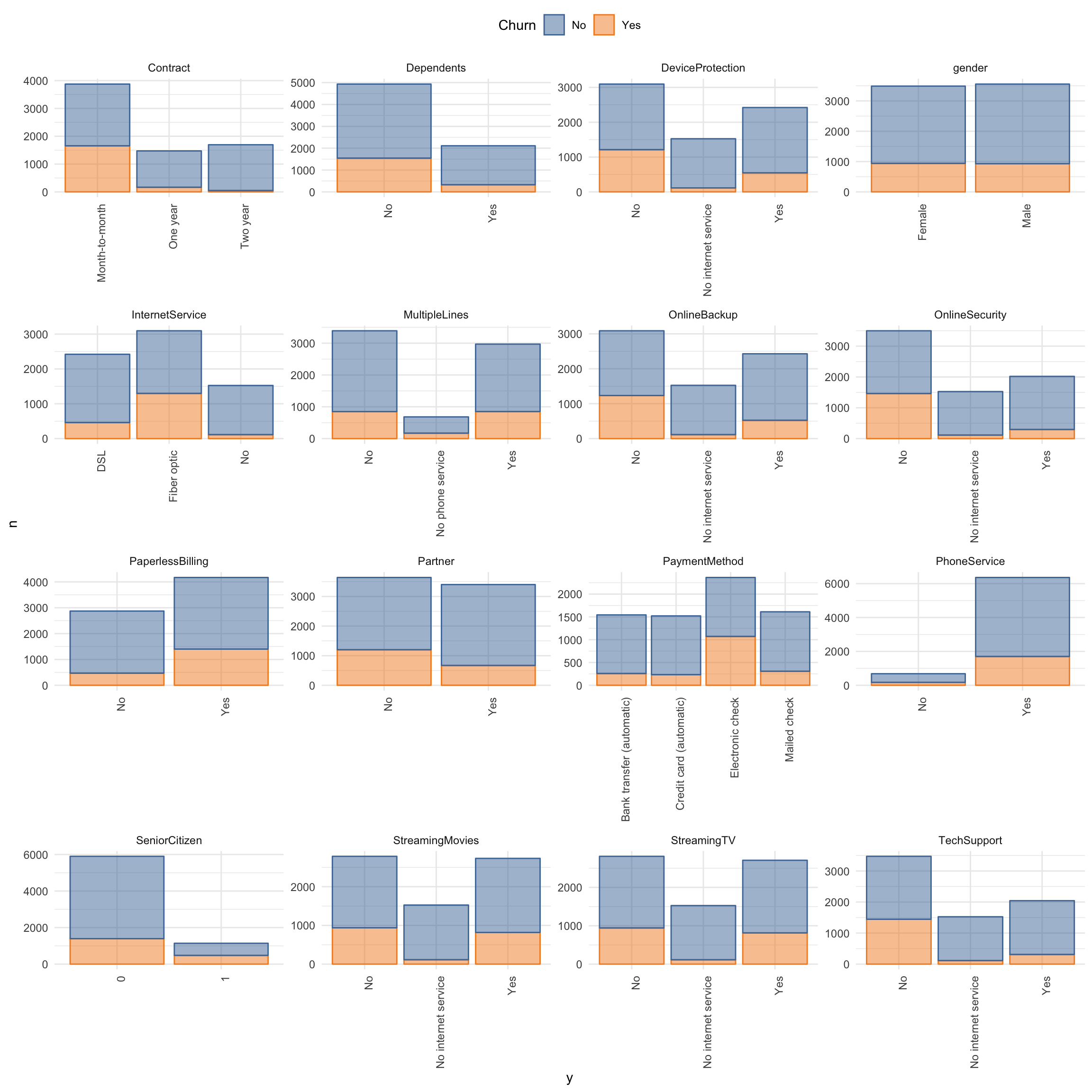
- Plot numerical features
churn_data_raw %>%
  select(-customerID) %>%
  #select_if(is.numeric) %>%
  select(Churn, MonthlyCharges, tenure, TotalCharges) %>%
  gather(x, y, MonthlyCharges:TotalCharges) %>%
  ggplot(aes(x = y, fill = Churn, color = Churn)) +
    facet_wrap(~ x, ncol = 3, scales = "free") +
    geom_density(alpha = 0.5) +
    theme(axis.text.x = element_text(angle = 90, hjust = 1),
          legend.position = "top") +
    scale_color_tableau() +
    scale_fill_tableau()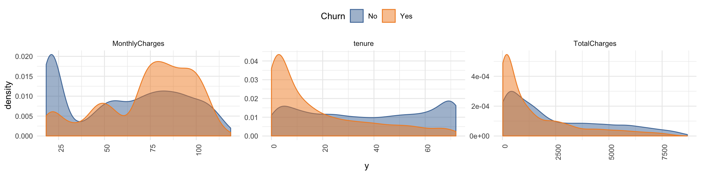
- Remove customer ID as it doesn’t provide information
churn_data <- churn_data_raw %>%
  select(-customerID)
Dealing with missing values
- Pattern of missing data
md.pattern(churn_data, plot = FALSE)## gender SeniorCitizen Partner Dependents tenure PhoneService
## 7032 1 1 1 1 1 1
## 11 1 1 1 1 1 1
## 0 0 0 0 0 0
## MultipleLines InternetService OnlineSecurity OnlineBackup
## 7032 1 1 1 1
## 11 1 1 1 1
## 0 0 0 0
## DeviceProtection TechSupport StreamingTV StreamingMovies Contract
## 7032 1 1 1 1 1
## 11 1 1 1 1 1
## 0 0 0 0 0
## PaperlessBilling PaymentMethod MonthlyCharges Churn TotalCharges
## 7032 1 1 1 1 1 0
## 11 1 1 1 1 0 1
## 0 0 0 0 11 11- Option 1: impute missing data => NOT done here!
imp <- mice(data = churn_data,  print = FALSE)
train_data_impute <- complete(imp, "long")- Option 2: drop missing data => done here because not too much information is lost by removing it
churn_data <- churn_data %>%
  drop_na()
Training and test split
- Partition data into training and test set
set.seed(42)
index <- createDataPartition(churn_data$Churn, p = 0.7, list = FALSE)- Partition test set again into validation and test set
train_data <- churn_data[index, ]
test_data  <- churn_data[-index, ]

index2 <- createDataPartition(test_data$Churn, p = 0.5, list = FALSE)

valid_data <- test_data[-index2, ]
test_data <- test_data[index2, ]nrow(train_data)## [1] 4924nrow(valid_data)## [1] 1054nrow(test_data)## [1] 1054Pre-Processing
- Create recipe for preprocessing
A recipe is a description of what steps should be applied to a data set in order to get it ready for data analysis.
recipe_churn <- recipe(Churn ~ ., train_data) %>%
  step_dummy(all_nominal(), -all_outcomes()) %>%
  step_center(all_predictors(), -all_outcomes()) %>%
  step_scale(all_predictors(), -all_outcomes()) %>%
prep(data = train_data)- Apply recipe to three datasets
train_data <- bake(recipe_churn, new_data = train_data) %>%
  select(Churn, everything())

valid_data <- bake(recipe_churn, new_data = valid_data) %>%
  select(Churn, everything())

test_data <- bake(recipe_churn, new_data = test_data) %>%
select(Churn, everything())- For Keras create response variable as one-hot encoded matrix
train_y_drop <- to_categorical(as.integer(as.factor(train_data$Churn)) - 1, 2)
colnames(train_y_drop) <- c("No", "Yes")

valid_y_drop <- to_categorical(as.integer(as.factor(valid_data$Churn)) - 1, 2)
colnames(valid_y_drop) <- c("No", "Yes")

test_y_drop <- to_categorical(as.integer(as.factor(test_data$Churn)) - 1, 2)
colnames(test_y_drop) <- c("No", "Yes")- Because we want to train on a binary outcome, we can delete the “No” column
# if training with binary crossentropy
train_y_drop <- train_y_drop[, 2, drop = FALSE]
head(train_y_drop)
## Yes
## [1,] 0
## [2,] 1
## [3,] 1
## [4,] 0
## [5,] 1
## [6,] 0valid_y_drop <- valid_y_drop[, 2, drop = FALSE]
test_y_drop <- test_y_drop[, 2, drop = FALSE]- Remove response variable from preprocessed data (for Keras)
train_data_bk <- select(train_data, -Churn)
head(train_data_bk)
## # A tibble: 6 x 30
## SeniorCitizen tenure MonthlyCharges TotalCharges gender_Male Partner_Yes
## <dbl> <dbl> <dbl> <dbl> <dbl> <dbl>
## 1 -0.439 0.0765 -0.256 -0.163 0.979 -0.966
## 2 -0.439 -1.23 -0.359 -0.949 0.979 -0.966
## 3 -0.439 -0.983 1.17 -0.635 -1.02 -0.966
## 4 -0.439 -0.901 -1.16 -0.863 -1.02 -0.966
## 5 -0.439 -0.168 1.34 0.347 -1.02 1.03
## 6 -0.439 1.22 -0.282 0.542 0.979 -0.966
## # ... with 24 more variables: Dependents_Yes <dbl>,
## # PhoneService_Yes <dbl>, MultipleLines_No.phone.service <dbl>,
## # MultipleLines_Yes <dbl>, InternetService_Fiber.optic <dbl>,
## # InternetService_No <dbl>, OnlineSecurity_No.internet.service <dbl>,
## # OnlineSecurity_Yes <dbl>, OnlineBackup_No.internet.service <dbl>,
## # OnlineBackup_Yes <dbl>, DeviceProtection_No.internet.service <dbl>,
## # DeviceProtection_Yes <dbl>, TechSupport_No.internet.service <dbl>,
## # TechSupport_Yes <dbl>, StreamingTV_No.internet.service <dbl>,
## # StreamingTV_Yes <dbl>, StreamingMovies_No.internet.service <dbl>,
## # StreamingMovies_Yes <dbl>, Contract_One.year <dbl>,
## # Contract_Two.year <dbl>, PaperlessBilling_Yes <dbl>,
## # PaymentMethod_Credit.card..automatic. <dbl>,
## # PaymentMethod_Electronic.check <dbl>, PaymentMethod_Mailed.check <dbl>valid_data_bk <- select(valid_data, -Churn)
test_data_bk <- select(test_data, -Churn)- Alternative to above, to convert response variable into numeric format where 1 = Yes and 0 = No
train_data$Churn <- ifelse(train_data$Churn == "Yes", 1, 0)
valid_data$Churn <- ifelse(valid_data$Churn == "Yes", 1, 0)
test_data$Churn <- ifelse(test_data$Churn == "Yes", 1, 0)
Modeling with Keras
- Define a simple MLP
model_keras <- keras_model_sequential()

model_keras %>%
  layer_dense(units = 32, kernel_initializer = "uniform", activation = "relu",
              input_shape = ncol(train_data_bk)) %>%
  layer_dropout(rate = 0.2) %>%

  layer_dense(units = 16, kernel_initializer = "uniform", activation = "relu") %>%
  layer_dropout(rate = 0.2) %>%

  layer_dense(units = 8, kernel_initializer = "uniform", activation = "relu") %>%
  layer_dropout(rate = 0.2) %>%

  layer_dense(units = 1,
              kernel_initializer = "uniform", activation = "sigmoid") %>%

  compile(
        optimizer = 'adamax',
        loss      = 'binary_crossentropy',
        metrics   = c("binary_accuracy", "mse")
    )

summary(model_keras)
## ___________________________________________________________________________
## Layer (type) Output Shape Param #
## ===========================================================================
## dense_1 (Dense) (None, 32) 992
## ___________________________________________________________________________
## dropout_1 (Dropout) (None, 32) 0
## ___________________________________________________________________________
## dense_2 (Dense) (None, 16) 528
## ___________________________________________________________________________
## dropout_2 (Dropout) (None, 16) 0
## ___________________________________________________________________________
## dense_3 (Dense) (None, 8) 136
## ___________________________________________________________________________
## dropout_3 (Dropout) (None, 8) 0
## ___________________________________________________________________________
## dense_4 (Dense) (None, 1) 9
## ===========================================================================
## Total params: 1,665
## Trainable params: 1,665
## Non-trainable params: 0
## ___________________________________________________________________________- Fit model (we could have used validation split on the trainings data instead of creating a validation set => see #)
fit_keras <- fit(model_keras,
    x = as.matrix(train_data_bk),
    y = train_y_drop,
    batch_size = 32,
    epochs = 20,
    #validation_split = 0.30,
    validation_data = list(as.matrix(valid_data_bk), valid_y_drop),
    verbose = 2
)- Plot Keras training results
plot(fit_keras) +
  scale_color_tableau() +
  scale_fill_tableau()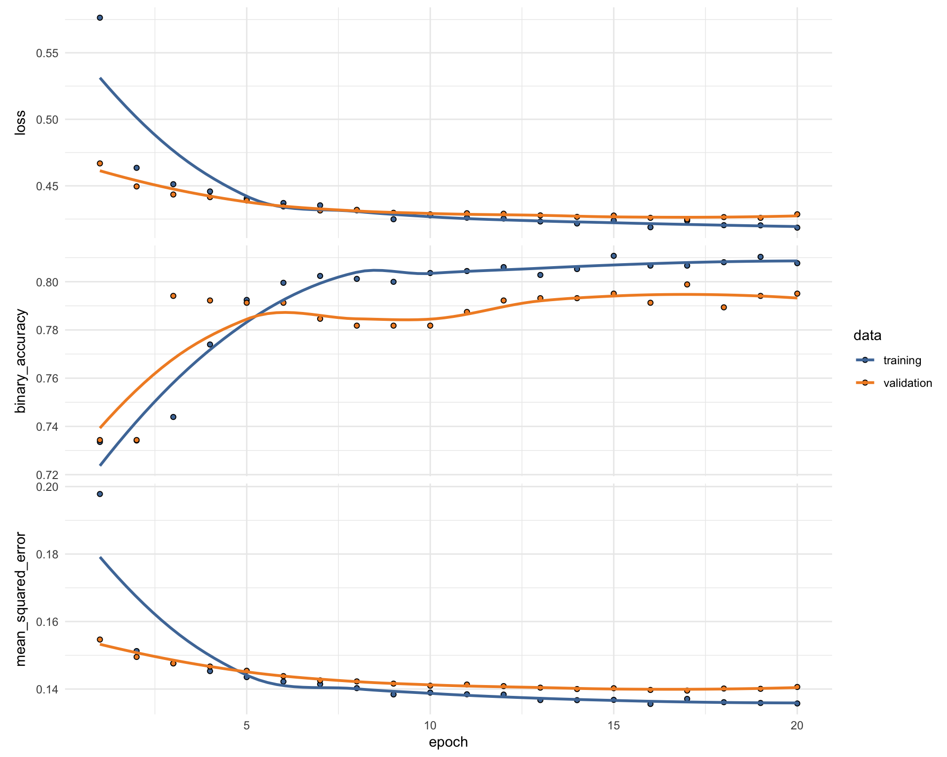
Evaluation
- Predict classes and probabilities
pred_classes_test <- predict_classes(object = model_keras, x = as.matrix(test_data_bk))
pred_proba_test <- predict_proba(object = model_keras, x = as.matrix(test_data_bk))- Create results table
test_results <- tibble(
  actual_yes = as.factor(as.vector(test_y_drop)),
  pred_classes_test = as.factor(as.vector(pred_classes_test)),
  Yes = as.vector(pred_proba_test),
  No = 1 - as.vector(pred_proba_test))
head(test_results)
## # A tibble: 6 x 4
## actual_yes pred_classes_test Yes No
## <fct> <fct> <dbl> <dbl>
## 1 0 1 0.516 0.484
## 2 0 0 0.0145 0.985
## 3 1 1 0.680 0.320
## 4 1 0 0.390 0.610
## 5 0 0 0.00610 0.994
## 6 0 0 0.0371 0.963- Calculate confusion matrix
test_results %>%
  conf_mat(actual_yes, pred_classes_test)
## Truth
## Prediction 0 1
## 0 697 128
## 1 77 152- Calculate metrics
test_results %>%
  metrics(actual_yes, pred_classes_test)
## # A tibble: 2 x 3
## .metric .estimator .estimate
## <chr> <chr> <dbl>
## 1 accuracy binary 0.806
## 2 kap binary 0.471- Are under the ROC curve
test_results %>%
  roc_auc(actual_yes, Yes)
## # A tibble: 1 x 3
## .metric .estimator .estimate
## <chr> <chr> <dbl>
## 1 roc_auc binary 0.840- Precision and recall
tibble(
    precision = test_results %>% yardstick::precision(actual_yes, pred_classes_test) %>% select(.estimate) %>% as.numeric(),
    recall    = test_results %>% yardstick::recall(actual_yes, pred_classes_test) %>% select(.estimate) %>% as.numeric()
)
## # A tibble: 1 x 2
## precision recall
## <dbl> <dbl>
## 1 0.845 0.901- F1-Statistic
test_results %>% yardstick::f_meas(actual_yes, pred_classes_test, beta = 1)## # A tibble: 1 x 3
## .metric .estimator .estimate
## <chr> <chr> <dbl>
## 1 f_meas binary 0.872H2O
Shows an alternative to Keras!
- Initialise H2O instance and convert data to h2o frame
library(h2o)
h2o.init(nthreads = -1)
## Connection successful!
##
## R is connected to the H2O cluster:
## H2O cluster uptime: 2 minutes 36 seconds
## H2O cluster timezone: Europe/Berlin
## H2O data parsing timezone: UTC
## H2O cluster version: 3.20.0.8
## H2O cluster version age: 3 months and 25 days !!!
## H2O cluster name: H2O_started_from_R_shiringlander_pir412
## H2O cluster total nodes: 1
## H2O cluster total memory: 3.47 GB
## H2O cluster total cores: 8
## H2O cluster allowed cores: 8
## H2O cluster healthy: TRUE
## H2O Connection ip: localhost
## H2O Connection port: 54321
## H2O Connection proxy: NA
## H2O Internal Security: FALSE
## H2O API Extensions: XGBoost, Algos, AutoML, Core V3, Core V4
## R Version: R version 3.5.1 (2018-07-02)h2o.no_progress()
train_hf <- as.h2o(train_data)
valid_hf <- as.h2o(valid_data)
test_hf <- as.h2o(test_data)
response <- "Churn"
features <- setdiff(colnames(train_hf), response)# For binary classification, response should be a factor
train_hf[, response] <- as.factor(train_hf[, response])
valid_hf[, response] <- as.factor(valid_hf[, response])
test_hf[, response] <- as.factor(test_hf[, response])summary(train_hf$Churn, exact_quantiles = TRUE)## Churn
## 0:3615
## 1:1309summary(valid_hf$Churn, exact_quantiles = TRUE)## Churn
## 0:774
## 1:280summary(test_hf$Churn, exact_quantiles = TRUE)## Churn
## 0:774
## 1:280- Train model with AutoML.
“During model training, you might find that the majority of your data belongs in a single class. For example, consider a binary classification model that has 100 rows, with 80 rows labeled as class 1 and the remaining 20 rows labeled as class 2. This is a common scenario, given that machine learning attempts to predict class 1 with the highest accuracy. It can also be an example of an imbalanced dataset, in this case, with a ratio of 4:1. The balance_classes option can be used to balance the class distribution. When enabled, H2O will either undersample the majority classes or oversample the minority classes. Note that the resulting model will also correct the final probabilities (“undo the sampling”) using a monotonic transform, so the predicted probabilities of the first model will differ from a second model. However, because AUC only cares about ordering, it won’t be affected. If this option is enabled, then you can also specify a value for the class_sampling_factors and max_after_balance_size options.” http://docs.h2o.ai/h2o/latest-stable/h2o-docs/data-science/algo-params/balance_classes.html
aml <- h2o.automl(x = features,
                  y = response,
                  training_frame = train_hf,
                  validation_frame = valid_hf,
                  balance_classes = TRUE,
                  max_runtime_secs = 3600)

# View the AutoML Leaderboard
lb <- aml@leaderboard

best_model <- aml@leader

h2o.saveModel(best_model, "/Users/shiringlander/Documents/Github/Data")- Prediction
pred <- h2o.predict(best_model, test_hf[, -1])- Mean per class error
h2o.mean_per_class_error(best_model, train = TRUE, valid = TRUE, xval = TRUE)## train valid xval
## 0.1717911 0.2172683 0.2350682- Confusion matrix on validation data
h2o.confusionMatrix(best_model, valid = TRUE)## Confusion Matrix (vertical: actual; across: predicted) for max f1 @ threshold = 0.258586059604449:
## 0 1 Error Rate
## 0 478 130 0.213816 =130/608
## 1 49 173 0.220721 =49/222
## Totals 527 303 0.215663 =179/830h2o.auc(best_model, train = TRUE)## [1] 0.9039696h2o.auc(best_model, valid = TRUE)## [1] 0.8509068h2o.auc(best_model, xval = TRUE)## [1] 0.8397085- Performance and confusion matrix on test data
perf <- h2o.performance(best_model, test_hf)
h2o.confusionMatrix(perf)
## Confusion Matrix (vertical: actual; across: predicted) for max f1 @ threshold = 0.40790847476229:
## 0 1 Error Rate
## 0 667 107 0.138243 =107/774
## 1 86 194 0.307143 =86/280
## Totals 753 301 0.183112 =193/1054- Plot performance
plot(perf)- More performance metrics extracted
h2o.logloss(perf)## [1] 0.4008041h2o.mse(perf)## [1] 0.1278505h2o.auc(perf)## [1] 0.8622301metrics <- as.data.frame(h2o.metric(perf))
head(metrics)## threshold f1 f2 f0point5 accuracy precision
## 1 0.8278177 0.01418440 0.008912656 0.03472222 0.7362429 1
## 2 0.8203439 0.02816901 0.017793594 0.06756757 0.7381404 1
## 3 0.8173635 0.04195804 0.026642984 0.09868421 0.7400380 1
## 4 0.8160146 0.04878049 0.031055901 0.11363636 0.7409867 1
## 5 0.8139018 0.05555556 0.035460993 0.12820513 0.7419355 1
## 6 0.8112067 0.07560137 0.048629531 0.16975309 0.7447818 1
## recall specificity absolute_mcc min_per_class_accuracy
## 1 0.007142857 1 0.07249342 0.007142857
## 2 0.014285714 1 0.10261877 0.014285714
## 3 0.021428571 1 0.12580168 0.021428571
## 4 0.025000000 1 0.13594622 0.025000000
## 5 0.028571429 1 0.14540208 0.028571429
## 6 0.039285714 1 0.17074408 0.039285714
## mean_per_class_accuracy tns fns fps tps tnr fnr fpr tpr
## 1 0.5035714 774 278 0 2 1 0.9928571 0 0.007142857
## 2 0.5071429 774 276 0 4 1 0.9857143 0 0.014285714
## 3 0.5107143 774 274 0 6 1 0.9785714 0 0.021428571
## 4 0.5125000 774 273 0 7 1 0.9750000 0 0.025000000
## 5 0.5142857 774 272 0 8 1 0.9714286 0 0.028571429
## 6 0.5196429 774 269 0 11 1 0.9607143 0 0.039285714
## idx
## 1 0
## 2 1
## 3 2
## 4 3
## 5 4
## 6 5- Plot performance metrics
metrics %>%
  gather(x, y, f1:tpr) %>%
  ggplot(aes(x = threshold, y = y, group = x)) +
    facet_wrap(~ x, ncol = 2, scales = "free") +
    geom_line()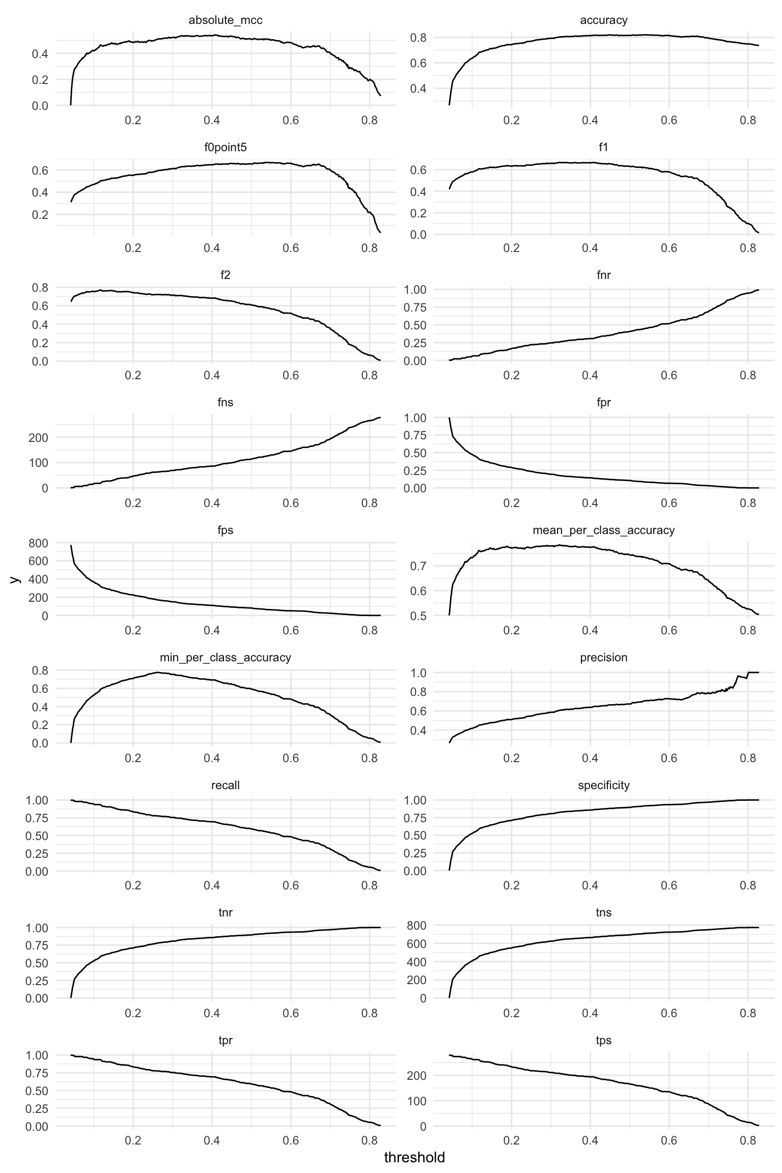
- Examine prediction thresholds
threshold <- metrics[order(-metrics$accuracy), "threshold"][1]

finalRf_predictions <- data.frame(actual = as.vector(test_hf$Churn),
                                  as.data.frame(h2o.predict(object = best_model,
                                                            newdata = test_hf)))
head(finalRf_predictions)
## actual predict p0 p1
## 1 0 1 0.3870607 0.61293929
## 2 0 0 0.9341973 0.06580274
## 3 1 1 0.2868668 0.71313316
## 4 1 1 0.3498788 0.65012119
## 5 0 0 0.9491335 0.05086646
## 6 0 0 0.9364659 0.06353410finalRf_predictions$accurate <- ifelse(finalRf_predictions$actual ==
finalRf_predictions$predict, "ja", "nein")
finalRf_predictions$predict_stringent <- ifelse(finalRf_predictions$p1 > threshold, 1,
ifelse(finalRf_predictions$p0 > threshold, 0, "unsicher"))
finalRf_predictions$accurate_stringent <- ifelse(finalRf_predictions$actual ==
finalRf_predictions$predict_stringent, "ja",
ifelse(finalRf_predictions$predict_stringent ==
"unsicher", "unsicher", "nein"))
finalRf_predictions %>%
group_by(actual, predict) %>%
dplyr::summarise(n = n())## # A tibble: 4 x 3
## # Groups: actual [?]
## actual predict n
## <fct> <fct> <int>
## 1 0 0 602
## 2 0 1 172
## 3 1 0 63
## 4 1 1 217finalRf_predictions %>%
group_by(actual, predict_stringent) %>%
dplyr::summarise(n = n())## # A tibble: 6 x 3
## # Groups: actual [?]
## actual predict_stringent n
## <fct> <chr> <int>
## 1 0 0 683
## 2 0 1 63
## 3 0 unsicher 28
## 4 1 0 101
## 5 1 1 152
## 6 1 unsicher 27finalRf_predictions %>%
gather(x, y, accurate, accurate_stringent) %>%
mutate(x = ifelse(x == "accurate", "Default Schwelle: 0.5",
paste("Angepasste Schwelle:", round(threshold, digits = 2)))) %>%
ggplot(aes(x = actual, fill = y)) +
facet_grid(~ x) +
geom_bar(position = "dodge") +
scale_fill_tableau()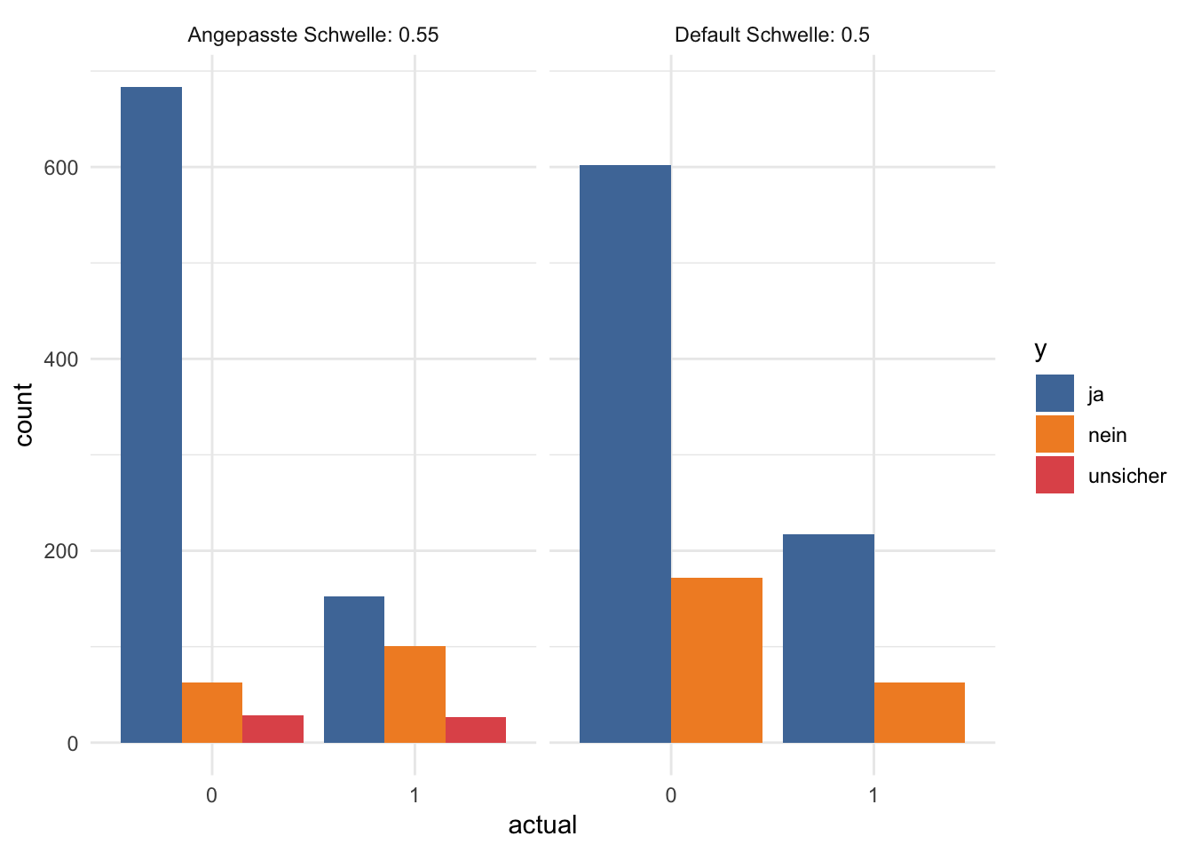
df <- finalRf_predictions[, c(1, 3, 4)]

thresholds <- seq(from = 0, to = 1, by = 0.1)

prop_table <- data.frame(threshold = thresholds,
                         prop_p0_true = NA, prop_p0_false = NA,
                         prop_p1_true = NA, prop_p1_false = NA)

for (threshold in thresholds) {

  pred_1 <- ifelse(df$p1 > threshold, 1, 0)
  pred_1_t <- ifelse(pred_1 == df$actual, TRUE, FALSE)

  group <- data.frame(df,
                      "pred_true" = pred_1_t) %>%
    group_by(actual, pred_true) %>%
    dplyr::summarise(n = n())

  group_p0 <- filter(group, actual == "0")

  prop_p0_t <- sum(filter(group_p0, pred_true == TRUE)$n) / sum(group_p0$n)
  prop_p0_f <- sum(filter(group_p0, pred_true == FALSE)$n) / sum(group_p0$n)
  prop_table[prop_table$threshold == threshold, "prop_p0_true"] <- prop_p0_t
  prop_table[prop_table$threshold == threshold, "prop_p0_false"] <- prop_p0_f

  group_p1 <- filter(group, actual == "1")

  prop_p1_t <- sum(filter(group_p1, pred_true == TRUE)$n) / sum(group_p1$n)
  prop_p1_f <- sum(filter(group_p1, pred_true == FALSE)$n) / sum(group_p1$n)
  prop_table[prop_table$threshold == threshold, "prop_p1_true"] <- prop_p1_t
  prop_table[prop_table$threshold == threshold, "prop_p1_false"] <- prop_p1_f
}
prop_table %>%
gather(x, y, prop_p0_true, prop_p1_true) %>%
rename(Schwellenwert = threshold) %>%
mutate(x = ifelse(x == "prop_p0_true", "prop true p0",
"prop true p1")) %>%
ggplot(aes(x = Schwellenwert, y = y, color = x)) +
geom_point() +
geom_line() +
scale_color_tableau()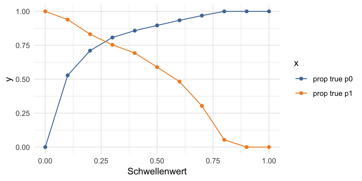
Cost/revenue calculation
Let’s assume that
- a marketing campaign + employee time will cost the company 1000€ per year for every customer that is included in the campaign.
- the annual average revenue per customer is 2000€ (in more complex scenarios customers could be further divided into revenue groups to calculate how “valuable” they are and how harmful loosing them would be)
- investing into unnecessary marketing doesn’t cause churn by itself (i.e. a customer who isn’t going to churn isn’t reacting negatively to the add campaign - which could happen in more complex scenarios).
- without a customer churn model the company would target half of their customer (by chance) for ad-campaigns
- without a customer churn model the company would lose about 25% of their customers to churn
This would mean that compared to no intervention we would have
- prop_p0_true == customers who were correctly predicted to not churn did not cost anything (no marketing money was spent): +/-0€
- prop_p0_false == customers that did not churn who are predicted to churn will be an empty investment: +/-0€ - 1500€
- prop_p1_false == customer that were predicted to stay but churned: -2000€
- prop_p1_true == customers that were correctly predicted to churn:
- let’s say 100% of those could be kept by investing into marketing: +2000€ -1500€
- let’s say 50% could be kept by investing into marketing: +2000€ * 0.5 -1500€
- Let’s play around with some values:
# Baseline
revenue <- 2000
cost <- 1000

customers_churn <- filter(test_data, Churn == 1)
customers_churn_n <- nrow(customers_churn)

customers_no_churn <- filter(filter(test_data, Churn == 0))
customers_no_churn_n <- nrow(customers_no_churn)

customers <- customers_churn_n + customers_no_churn_n

ad_target_rate <- 0.5
ad_cost_default <- customers * ad_target_rate * cost

churn_rate_default <- customers_churn_n / customers_no_churn_n
ann_revenue_default <- customers_no_churn_n * revenue

net_win_default <- ann_revenue_default - ad_cost_default
net_win_default
## [1] 1021000- How much revenue can we gain from predicting customer churn (assuming conversionr rate of 0.7):
conversion <- 0.7

net_win_table <- prop_table %>%
  mutate(prop_p0_true_X = prop_p0_true * customers_no_churn_n * revenue,
         prop_p0_false_X = prop_p0_false * customers_no_churn_n * (revenue -cost),
         prop_p1_false_X = prop_p1_false * customers_churn_n * 0,
         prop_p1_true_X = prop_p1_true * customers_churn_n * ((revenue * conversion) - cost)) %>%
  group_by(threshold) %>%
  summarise(net_win = sum(prop_p0_true_X + prop_p0_false_X + prop_p1_false_X + prop_p1_true_X),
            net_win_compared = net_win - net_win_default) %>%
  arrange(-net_win_compared)

net_win_table
## # A tibble: 11 x 3
## threshold net_win net_win_compared
## <dbl> <dbl> <dbl>
## 1 0.7 1558000 537000
## 2 0.8 1554000 533000
## 3 0.6 1551000 530000
## 4 0.9 1548000 527000
## 5 1 1548000 527000
## 6 0.5 1534000 513000
## 7 0.4 1515600 494600
## 8 0.3 1483400 462400
## 9 0.2 1417200 396200
## 10 0.1 1288200 267200
## 11 0 886000 -135000LIME
- Explaining predictions
Xtrain <- as.data.frame(train_hf)
Xtest <- as.data.frame(test_hf)

# run lime() on training set
explainer <- lime::lime(x = Xtrain,
                        model = best_model)

# run explain() on the explainer
explanation <- lime::explain(x = Xtest[1:9, ],
                             explainer = explainer,
                             n_labels = 1,
                             n_features = 4,
                             kernel_width = 0.5)
plot_explanations(explanation)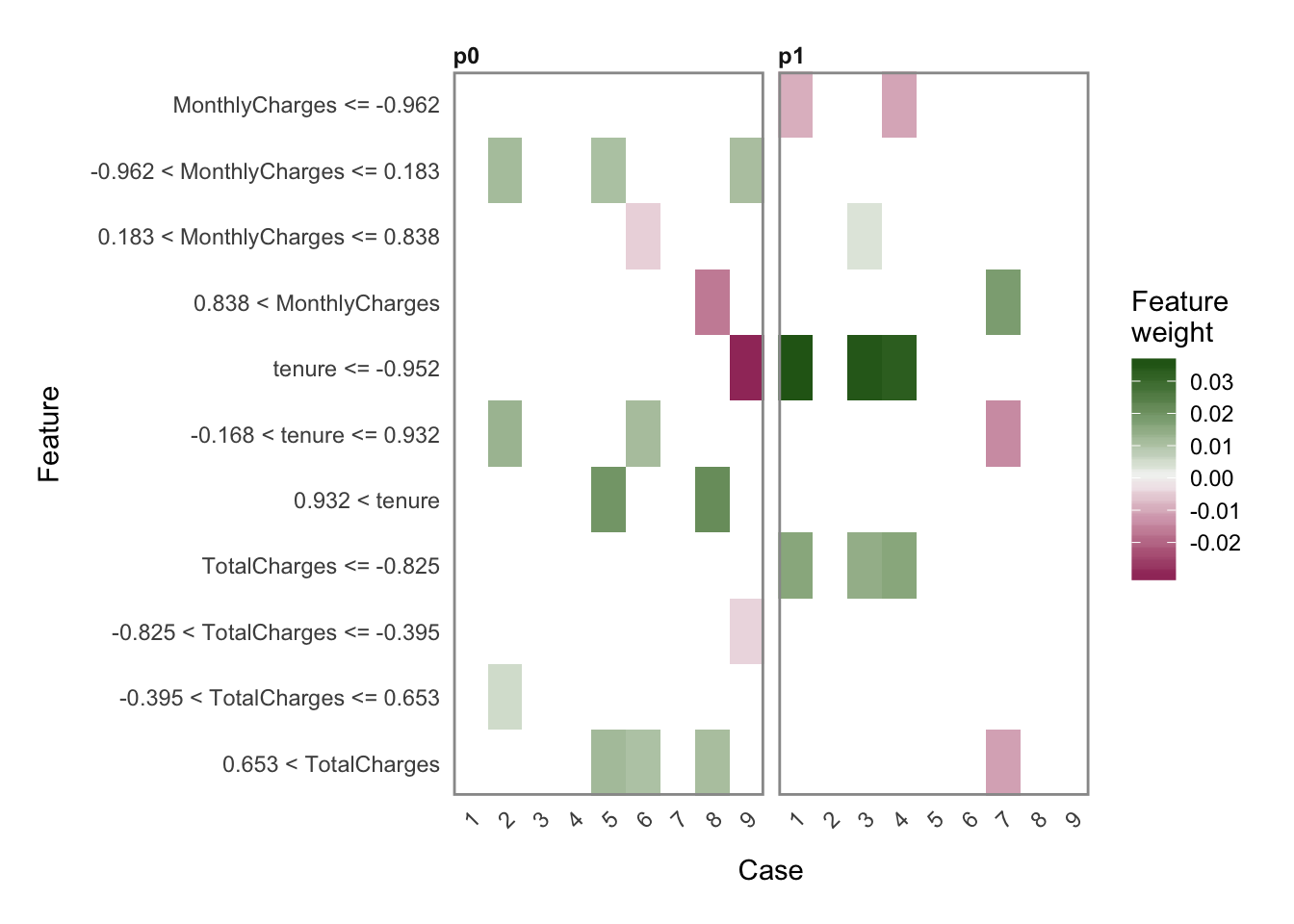
explanation %>%
  plot_features(ncol = 3)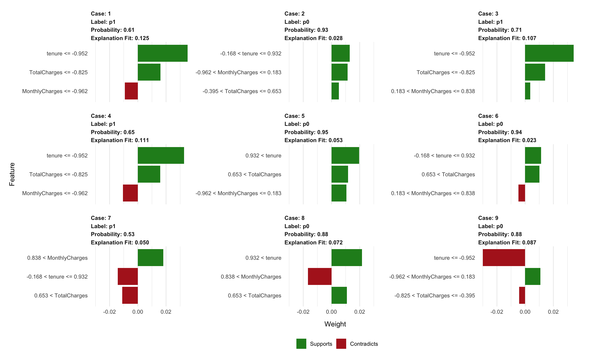
sessionInfo()## R version 3.5.1 (2018-07-02)
## Platform: x86_64-apple-darwin15.6.0 (64-bit)
## Running under: macOS 10.14.2
##
## Matrix products: default
## BLAS: /Library/Frameworks/R.framework/Versions/3.5/Resources/lib/libRblas.0.dylib
## LAPACK: /Library/Frameworks/R.framework/Versions/3.5/Resources/lib/libRlapack.dylib
##
## locale:
## [1] en_US.UTF-8/en_US.UTF-8/en_US.UTF-8/C/en_US.UTF-8/en_US.UTF-8
##
## attached base packages:
## [1] stats graphics grDevices utils datasets methods base
##
## other attached packages:
## [1] h2o_3.20.0.8 bindrcpp_0.2.2 corrplot_0.84 ggthemes_4.0.1
## [5] yardstick_0.0.2 recipes_0.1.4 rsample_0.0.3 lime_0.4.1
## [9] keras_2.2.4 mice_3.3.0 caret_6.0-81 lattice_0.20-38
## [13] forcats_0.3.0 stringr_1.3.1 dplyr_0.7.8 purrr_0.2.5
## [17] readr_1.3.1 tidyr_0.8.2 tibble_1.4.2 ggplot2_3.1.0
## [21] tidyverse_1.2.1
##
## loaded via a namespace (and not attached):
## [1] minqa_1.2.4 colorspace_1.3-2 class_7.3-15
## [4] base64enc_0.1-3 rstudioapi_0.8 prodlim_2018.04.18
## [7] fansi_0.4.0 lubridate_1.7.4 xml2_1.2.0
## [10] codetools_0.2-16 splines_3.5.1 knitr_1.21
## [13] shinythemes_1.1.2 zeallot_0.1.0 jsonlite_1.6
## [16] nloptr_1.2.1 pROC_1.13.0 broom_0.5.1
## [19] tfruns_1.4 shiny_1.2.0 compiler_3.5.1
## [22] httr_1.4.0 backports_1.1.3 assertthat_0.2.0
## [25] Matrix_1.2-15 lazyeval_0.2.1 cli_1.0.1
## [28] later_0.7.5 htmltools_0.3.6 tools_3.5.1
## [31] gtable_0.2.0 glue_1.3.0 reshape2_1.4.3
## [34] Rcpp_1.0.0 cellranger_1.1.0 nlme_3.1-137
## [37] blogdown_0.9 iterators_1.0.10 timeDate_3043.102
## [40] gower_0.1.2 xfun_0.4 lme4_1.1-19
## [43] rvest_0.3.2 mime_0.6 pan_1.6
## [46] MASS_7.3-51.1 scales_1.0.0 ipred_0.9-8
## [49] hms_0.4.2 promises_1.0.1 parallel_3.5.1
## [52] yaml_2.2.0 reticulate_1.10 rpart_4.1-13
## [55] stringi_1.2.4 tensorflow_1.10 foreach_1.4.4
## [58] lava_1.6.4 bitops_1.0-6 rlang_0.3.0.1
## [61] pkgconfig_2.0.2 evaluate_0.12 bindr_0.1.1
## [64] labeling_0.3 htmlwidgets_1.3 tidyselect_0.2.5
## [67] plyr_1.8.4 magrittr_1.5 bookdown_0.9
## [70] R6_2.3.0 generics_0.0.2 mitml_0.3-6
## [73] pillar_1.3.1 haven_2.0.0 whisker_0.3-2
## [76] withr_2.1.2 RCurl_1.95-4.11 survival_2.43-3
## [79] nnet_7.3-12 modelr_0.1.2 crayon_1.3.4
## [82] jomo_2.6-5 utf8_1.1.4 rmarkdown_1.11
## [85] grid_3.5.1 readxl_1.2.0 data.table_1.11.8
## [88] ModelMetrics_1.2.2 digest_0.6.18 xtable_1.8-3
## [91] httpuv_1.4.5.1 stats4_3.5.1 munsell_0.5.0
## [94] glmnet_2.0-16